Graphics CODEx
A collection of (graphics) programming reference documents
Graphics Pipeline
- Overview
- Input Assembly
- Vertex Shader
- Primitive Assembly
- Rasterisation
- Early Depth Test
- Pixel Shader
- Late Depth Test
- Output Merger
Overview
The Graphics Pipeline is the most complicated pipeline out of the three major pipelines. It is also the oldest pipeline and has evolved a lot over the many years. However, the basic concepts have remain unchanged from the original 3D rendering days of Wolftenstein 3D.
When we talk about rendering into a texture, this includes rendering to the display as well. The display is effectively just a texture that is being displayed on the screen, so the same logic holds.
You can see all of the different graphics pipeline stages in the diagram below. All stages coloured yellow are fixed function while all stages coloured green are programmable function

Input Assembly
Vertex and Index Data
Each model is represented by two sets of data, the vertex and index data.
The vertex data is the data for the set of points, or vertices that make up a 3D model. At the very minimum, the vertex data must hold the positional representation of the point. Often extra data is associated with a vertex as well such as the normal, texture coordinate(s), tangent(s), vertex colour(s), skinning weight(s), etc.
The index data is a sequential list of indices that indicate which vertices link together to form a triangle. By separating the representation of which vertices form a triangle, we can re-use vertices across triangles. In general, there are three types of ways to represent triangles in an index sequence: list, strip and fan.
Triangle List is the simplest concept, where each triangle is made up by 3 indices within the index buffer. This is the simplest
way of representing triangle indices, but is also the least efficient way as we aren’t re-using any indices. In order to represent
N triangles, we need 3 * N indices in our index sequence.

int indices[] =
{
	0, 1, 2, // Triangle 0
	1, 2, 3, // Triangle 1
	2, 3, 4  // Triangle 2
};
Triangle Strip is the most common used concept, where each triangle re-uses the last two indices of the previously described triangle.
Only the first triangle uses three indices, all other triangles described afterwards only needs a single index as it re-uses the previous two.
As a result, in order to represent N triangles, we need 2 + N indices in our index sequence. This means that triangle strip uses only
~33% of indices compared to triangle list, resulting in a significant memory usage reduction.
int indices[] =
{
	0, 1, 2, // Triangle 0
	3,       // Triangle 1 (re-uses 1, 2)
	4        // Triangle 2 (re-uses 2, 3)
};
Triangle Fan is the least used one. It has the same memory cost as triangle strip but has the added benefit of implicitly providing
adjacency information, which can be used for certain optimisation or visual techniques. However, the amount of calculation work required
to represent a model in this format often outweighs the benefits, to the point where this method has even been deprecated in
more modern graphics API’s. The basic idea is that a single index describes the centre vertex of a fan, with all following indices
describing triangles connected to the centre vertex forming a fan around said vertex. As a result, in order to represent N triangles,
we need 2 + N indices in our index sequence.

int indices[] =
{
	0, // Centre vertex
	1, // First connecting vertex
	2, // Triangle 0 (re-uses 0, 1)
	3, // Triangle 1 (re-uses 0, 2)
	4, // Triangle 2 (re-uses 0, 3)
	...
};
Input Assembly Stage
The Input Assembly is the first stage in the Graphics Pipeline. This is a fixed function stage and is responsible for gathering and preparing all of the data that we want to send to the vertex shader. The input assembly fetches the per-vertex and per-instance data from the buffers that declared and bound by the graphics programmer through the graphics API and ensures that the data is in memory ready for the vertex shader to start execution.
The graphics programmer binds one or more buffers1, called vertex buffers to the graphics pipeline and tells the input assembly state how to read the data from said buffer(s).
// Pseudocode
struct VertexData
{
	vec3 Position;
	vec3 Normal;
};
VertexData vertexData[] = { ... };

struct InstanceData
{
	mat4 WorldTransform;
};
InstanceData instanceData[] = { ... };

// Bind our buffer(s)
InputAssembly.SetVertexBufer( 0u /* BufferIndex */, vertexData );
InputAssembly.SetVertexBufer( 1u /* BufferIndex */, instanceData );

// Describe how to read the data from the buffer(s)
InputAssembly.VertexAttribute( 0u /* AttributeIndex */, 0u /* BufferIndex */, offsetof( VertexData::Position ) /* Offset */, sizeof( VertexData::Position ) /* Stride */, PerVertex );
InputAssembly.VertexAttribute( 1u /* AttributeIndex */, 0u /* BufferIndex */, offsetof( VertexData::Normal ) /* Offset */, sizeof( VertexData::Normal ) /* Stride */, PerVertex );
InputAssembly.VertexAttribute( 2u /* AttributeIndex */, 1u /* BufferIndex */, offsetof( InstanceData::WorldTransform ) /* Offset */, sizeof( InstanceData::WorldTransform ) /* Stride */, PerInstance );
Vertex Shader
The vertex shader is ran once for every vertex within a model and is responsible for calculating the 2D clip space position for the vertex, explained more in the Transforms section. Even though the clip space position is the only requirement, the vertex shader also calculates any other values required for later in the pipeline, such as the world normals. This stage is a programmable stage.
Transforms
When talking about 3D, we see our data in an imaginary 3D space. However, displays are a 2D plane. As a result, we need to apply a set of transforms to go from the 3D positional data to a 2D projected plane. This is done through a series of matrix transforms.
World
When we have our vertex and index data of a model loaded, the positional data of the vertices are relative to the origin of the model,
often called the pivot point. However, if we would just render the model as-is, that would mean that every model would be orientated
the exact same way and be placed at the world origin, or the (0, 0, 0) location. This is of course not desired, so we need to apply a transform
to the model in order to place it and orientate it as we desire. This transform is called the world transform. The world transform is usually
a simple affine transformation matrix consisting of translation, rotation and scale. Once we have applied the world transform to the positional
data of the model, it is said that the model is in world space.

View
Once we have our models transformed to world space, we need to be able to determine where we are viewing them from. This is effectively the information of where the camera is placed within our world and which direction it is looking. In order to have our model positional data be relative to the camera position, we need to transform them with the view transform. This is also usually a simple affine transformation matrix consisting of translation and rotation. Once we have applied the view transform to the world space positional data, it is said that the model is in view space.
Projection
We now have our model data relative to our camera location, but we are still representing our data in a 3D space. Because we need to end up with
a 2D representation of our data, we need to project our data onto the viewing plane. This is done through the projection transform. This is a
non-affine transformation that through some very clever maths calculates the 2D projection of a point from a 3D space and transforms them to the [-1, 1] range.
Once we have applied the projection transform, it is said that the model is in clip space.
The X and Y dimensions of clip space are in the
[-1, 1]range. The Z dimension can be either[0, 1](DirectX) or[-1, 1](OpenGL) range depending on which graphics API is being used. The orientations of these values also differ between the different graphics API’s, with DirectX having the convention of(-1,-1)representing the bottom-left corner of the plane while in OpenGL the(-1, -1)represents the top-left corner.
struct VertexInput
{
	vec3 LocalPosition;       // PerVertex
	vec3 LocalNormal;         // PerVertex
	mat4 WorldTransform; // PerInstance
};

struct VertexOutput
{
	vec3 WorldPosition
	vec3 WorldNormal;
	vec3 ClipPosition;
};

void VertexShader
(
	/* in */  mat4 viewProjectionTransform,
	/* in */  VertexInput input
	/* out */ VertexOutput output
)
{
	output.WorldPosition = input.LocalPosition * input.WorldTransform;
	output.WorldNormal = input.LocalNormal * input.WorldTransform;
	output.ClipPosition = output.WorldPosition * viewProjectionTransform;
}
Primitive Assembly
Once all of the vertices have been projected and their clip space positions calculated, we can use the index data to connect the projected vertices into projected triangles. Older GPU’s used to support point and line rendering as well, which is why we call these primitives and not just triangles. However, these days point and line rendering is all emulated through triangle rendering and are barely ever used.
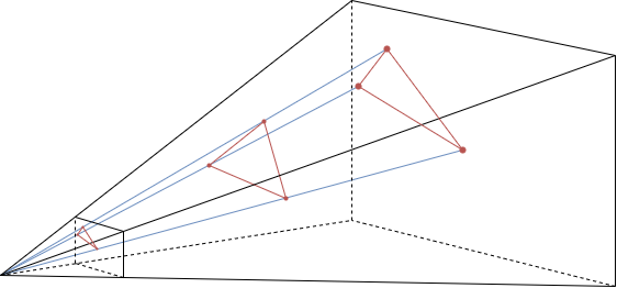
View culling & clipping
Because we now have the triangles projected onto the 2D plane, we know which triangles fall fully inside the viewing plane, which ones fall fully outside and which ones intersect the edges.
In this image you can see three types of triangles. The ones that are inside the viewing plane are sent through without modification. The ones that are outside the viewing plane are discarded by the hardware and stop being processed as they can never affect the final texture, so there’s no point in continuing to process them. This process is called culling.
There is also a third type, where a triangle is partially inside the viewing plane. These triangles are subdivided into the part that is inside the viewing plane and the part that is outside the viewing plane. The part that is outside is discarded and the part that is inside is sent through as a newly generated primitive. This process is called clipping.
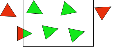
Front and back face culling
At this point in time the hardware can also deduce if a triangle is front-facing or back-facing. When we specify our vertices in
the index buffer, we can specify them in any order we want. For instance, we can specify them as 0, 1, 2, 0, 2, 1, 1, 2, 0, …
This sequence indicates the order in which we consider the vertices to form the triangle.

When the triangle has then been projected onto our viewing plane, we can check how this sequence represents on the 2D plane. It can either be projected in a clockwise order, or a counter-clockwise order. We can tell the primitive assembler which one of these two we consider front-facing and which one we consider back-facing.
In the example above, if we specified our vertex indices as 0, 1, 2 and consider clockwise front-facing, then the triangle on the left
is a back-facing triangle and the triangle on the right is front-facing.
Just because a triangle is front-facing or back-facing does not automatically qualify it to be culled. Similarly to how we can tell the primitive assembler which one we consider front or back, we can also tell it what we want to do with this information. The three states that are generally supported are cull back face, cull front face and cull none. Back face culling is considered the default state that should be used for rendering, but the other two states are often used to achieve specific visual effects, such as using cull none to achieve two-sided materials.
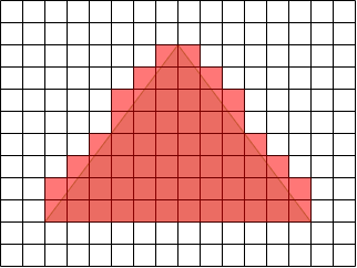
Rasterisation
We now have our model projected onto the 2D viewing plane. This viewing plane does not have a finite resolution though. You can see this plane as a raster (grid) where each cell within the grid is infinitesimally small in size. However, the textures that we render to (or the display) do have a finite resolution, defined by the rendering resolution (e.g. 1920x1080). As a result, we need to quantise these projected values from the infinite grid to the finite grid. This process is called rasterisation.
Barycentric Coordinates
Once we have rasterised the 2D projection of our model, we know which pixels of our final texture they overlap with. However, we only have
data that has been calculated on a per-vertex basis, but we want to determine which data to use per-pixel in order to calculate the colour
values to output. This can be done through barycentric coordinates. Very simply explained, barycentric coordinates allow us to calculate
where in on a triangle surface a point is located. This location is expressed as a set of normalised weights, u, v and w.
Based on these weights, we can then do a weighted sum of the values corresponding to the three vertices forming the triangle in
order to get a representation of what the data would represent at that point on the triangle surface.

You will often see barycentric coordinates described with only
uandvcomponents. This is because barycentric coordinates are normalised. This means thatu + v + w = 1. As a result,wcan be derived as1 - u - v, meaning that we don’t have to store thewcomponent.
For a more detailed explanation, see this Scratchapixel article
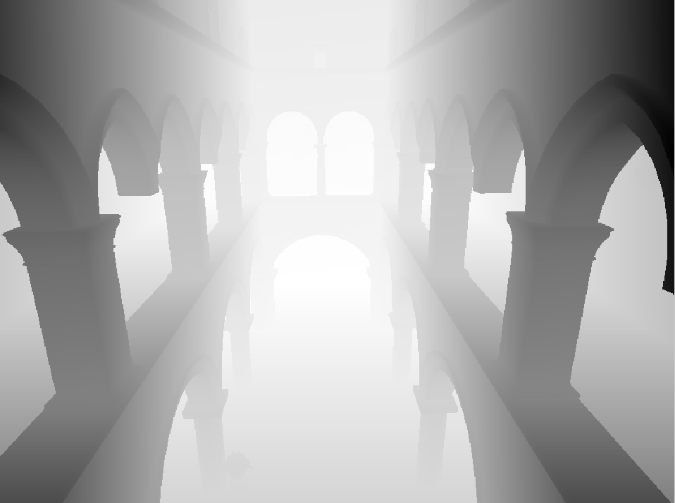
Early Depth Test
When we talk about having our vertices projected onto the 2D plane, we technically only use the x and y coordinates for placement.
However, we also calculated the depth z value. This value isn’t used for visual representation, but is only used in order to determine
how triangles are layered on top of each other.
When rendering with depth testing enabled, we not only render into a colour texture, we also rendering into a texture holding the depth values for each pixel, called the depth (stencil) buffer2.
Depth testing is done per-pixel, with the z value for a pixel being calculated through the barycentric coordinates
of the vertices of the triangle for which we’re calculating the new pixel value.
When a pixel is being depth tested, the depth value that exists for that pixel in the depth buffer is read and compared to the newly calculated depth value. When the depth test passes, the new value is written to the depth buffer and operation continues (e.g. writing colour value to colour buffer). If the depth test fails, no new value is written and the newly calculated pixel is rejected.
The depth test is often implemented as a simple less-equal comparison, but can be configured by the programmer using the graphics API in order to achieve different visual effects (e.g. using inverted depth buffer which requires greater-equal as comparison).
Before we run the pixel shader, we can execute an initial initial depth test. If a pixel fails the depth test, we can avoid running the pixel shader as we know in advance that the late depth test would fail anyway, saving us precious processing time. This early depth test will only run if the following conditions hold true3:
- The pixel shader does not modify the depth value
- The pixel shader does not use any pixel-kill operations (e.g.
discard) - Alpha blending is disabled
Pixel Shader
The pixel shader runs once per-pixel and is responsible for calculating the final colour that we want to write to the final texture. This is where often the more expensive calculations are done, such as normal mapping, lighting calculations, etc.
The pixel shader is often one of the most complex parts of the rendering pipeline, but because this is a programmable stage, a lot of the special functionality has more to do with how shaders are executed, which would require an entire document of their own in order to properly explain.
struct PixelInput
{
	vec3 ClipPosition;
	vec3 WorldPosition;
	vec3 WorldNormal;
};

struct PixelOutput
{
	vec4 Colour;
};

void PixelShader
(
	/* in */  PixelInput input
	/* out */ PixelOutput output
)
{
	output.Colour = CalculateColour( input.WorldPosition, input.WorldNormal );
}
Late Depth Test
If the early depth test didn’t manage to depth test for a given pixel, the depth testing needs to happen after the pixel shader. This most often occurs when using alpha clip or alpha blend materials. If the depth test fails, the calculated colour value is discard. Else if the depth test passes, the calculated colour value is passed to the output merger.
Output Merger
The output merger is responsible for writing the calculated colour value from the pixel shader to the colour buffer(s). It is a fixed function stage. One of the states that can be controlled within this stage is the alpha blend state. This state controls how different colour values should be blended together in the event that a pixel has a colour value calculated for it multiple times.
The behaviour of the output merger is slightly different depending on if the alpha blend state is enabled or not. If the alpha blend state is disabled, the colour value is simply written to the colour buffer. However, if the alpha blend state is enabled, the output merger reads the colour value that already exists in the colour buffer and executes the blending function before writing out the newly calculated value.
Blend Function
The blending function is a simple mathematical function that can be controlled through the alpha blend state by the programmer
through the graphics API. The blend function is executed independently for the colour values rgb and alpha values a.
dest = composeFunc( srcFactor * srcValue, destFactor * destValue );
The following two components cannot be controlled by the state:
-
srcValue: The new value calculated by the pixel shader (
rgbora). -
destValue: The value that is already present in the colour buffer (
rgbora)
The following three components can be controlled by the state:
- srcFactor: A multiplier to use against the srcValue. Examples of this are Source Alpha, One, Source Colour, …
- destFactor: A multiplier to use against the destValue. Examples of this are 1 - Source Alpha, One, Dest Colour, …
- composeFunc: The function to use to compose the two new values together into a final value. These are usually Add, Subtract, Reverse Subtract, Min or Max.
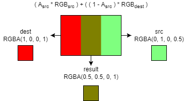
By controlling these different state elements, the programmer can affect how a newly calculated colour value gets written to the colour buffer. A common example for this is standard alpha blending:
dest.rgb = ( src.a * src.rgb ) + ( ( 1.0 - src.a ) * dest.rgb );
dest.a = 1.0;
You can see this formula as a linear interpolation between the colour already present and the newly calculated colour weighted by the alpha of the newly calculated colour. This results in a visual result where the new colour is layered on top of the existing colour and shifts the colour underneath, resulting in what looks like translucency.
-
Technically speaking we can also bind no vertex buffers and run the vertex shader without any pre-fetched data. This is sometimes done when all data is fetched from external buffers manually within the vertex shader. ↩
-
The stencil is a small texture bound together with the depth buffer that is often used for masking in/out rendering. ↩
-
Some other graphics API-specific features can also cause early depth testing to be disabled. ↩
Last modified on Wednesday 09 March 2022 at 20:36:42